PCA before DESeq2: the 30-second sanity check that catches what DE misses
Running PCA before differential expression takes 30 seconds and catches batch effects, mislabeled samples, and outliers that silently destroy DESeq2 results. How to read it.
If you go straight from counts to DESeq() without running PCA first, you don’t know what you’re testing.
I mean that literally. DESeq2 will happily fit its model, return p-values, and rank thousands of genes for you. The output will look exactly the same whether your strongest signal is the biological condition you care about, the date the libraries were prepped, or the fact that one sample is mislabeled. The function gives you the same numbers — they just mean radically different things.
PCA before DE is the 30-second check that tells you which case you’re in.
The 30 seconds of code that saves the analysis
Assume you already have a DESeqDataSet called dds. Before you call DESeq(dds), run:
vsd <- vst(dds, blind = TRUE)
plotPCA(vsd, intgroup = c("condition", "batch"))
That’s it. Two lines. vst() does a variance-stabilising transform that prevents high-expression genes from dominating the geometry. plotPCA() projects the top 500 most-variable genes onto the first two principal components and colours by whichever metadata columns you pass.
blind = TRUE is deliberate — you want the transformation to be agnostic to your design, so the PCA reflects what the data says, not what you’ve told the model to find.
What PCA is actually telling you
The mental shortcut “samples that cluster together are similar” is true but it misses the point. PCA is showing you the variance hierarchy of your dataset:
- PC1 = the single direction in expression space that explains the most variance across your samples. By construction, nothing explains more.
- PC2 = the next direction, orthogonal to PC1, that explains the second-most.
If your biological condition is real and meaningful, it should be the dominant axis of variation. PC1 should separate it cleanly. If PC1 separates anything else — sequencing batch, library prep date, the technician who ran the gels — then that is the strongest signal in your data, and your DE results are going to reflect it whether you want them to or not.
This is the whole reason intgroup = c("condition", "batch") matters: you want to see whether the same samples cluster the same way when you re-colour them by something technical.
Four failure modes PCA catches before DE
In order of how often they catch us:
1. Mislabeled samples
You see four clean clusters by condition, except one sample sits inside the wrong cluster. That’s a mislabel — the metadata calls it “treated” but the expression profile looks “control”, or vice versa.
This happens more often than people admit. Bench logs get mixed up; a sample swap during library prep doesn’t always get documented; the wrong tube gets indexed. PCA finds it in seconds. DESeq2 will not.
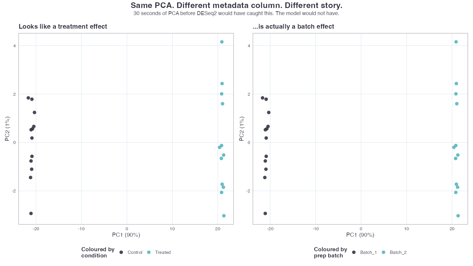
2. Batch effects masquerading as biology
The pathological case: PC1 separates conditions beautifully, but the conditions were also prepped on different days. When you re-colour by prep_date, you get the exact same separation along PC1.
You cannot tell from the DE p-values whether you’re looking at biology or batch. The model just sees a coherent signal. This is where post-hoc panics start, because the “discovery” was real, just not the discovery you thought.
3. Technical outliers
One sample sits alone in PC2, far from everyone else. Sometimes it’s a real biological outlier; more often it’s a technical one — degraded RNA, a failed library, a contaminated lane. Including it in DE pulls the dispersion estimates everywhere it shouldn’t.
4. The condition isn’t the dominant signal
PC1 separates by sex. PC2 separates by sample storage time. Your treatment vs. control shows up faintly on PC3. This isn’t necessarily fatal — DESeq2 can model the nuisance variables out — but it tells you something important: the biological effect you came here to measure is smaller than several other things. That changes how you interpret every downstream result.
What to do for each failure mode
| What PCA shows | What to do |
|---|---|
| One sample with the wrong colour | Confirm the metadata, fix the label, re-run. Do not silently drop. |
Same separation by condition and batch | Add batch to the design formula (~ batch + condition), or use ComBat-Seq if batches are unbalanced. If batches are completely confounded with condition, you do not have a salvageable experiment. |
| Lone sample in PC2 | Investigate: was there a QC flag in fastp? Low alignment rate? Adapter contamination? Drop only if you can name the technical reason. |
| Condition shows up on PC3 or later | Reconsider the design. Test the nuisance variables explicitly. Ask whether n is large enough to detect what you came to detect. |
Everything in this table is reversible and cheap before you commit to a DE model. The same fixes after DE are expensive, embarrassing, and sometimes impossible.
When PCA looks clean and you still have problems
PCA is not a complete QC — it’s the cheapest one. Things it can miss:
- Composition shifts. Two libraries with identical biological content but very different library complexity can produce subtly different fold-change estimates. PCA may not show it.
- Very low n. With three samples per group, “clean separation” can be coincidence. PCA looks reassuring but the inference is fragile.
- Genes with extreme dispersion. DESeq2 handles this internally, but if a handful of genes drive most of the variance you see on PC1, the picture can be misleading. Plot the gene loadings if PC1 looks suspiciously dominated by one tail.
These cases need DESeq2’s internal diagnostics — dispersion plots, MA plots, the lfcShrink() output — not just PCA. But every one of them is easier to spot when you already know what the PCA looked like.
The takeaway
Two lines of R, run before DESeq(), will save you from publishing a batch effect, chasing a mislabel, or interpreting an outlier as biology. There is no version of this analysis where skipping that step is the right call.
If you have RNA-seq data sitting on a server and you want someone else to do this for you properly — including the PCA before any DE runs, with the figures attached to the report — upload FASTQs to omicsdesk.com. The intake agent confirms the analysis plan with you before anything runs, the QC and PCA are part of every deliverable, and the timeline is fixed at 7–10 business days.