RNA-seq from FASTQ to DE: what a reproducible pipeline actually looks like in 2026
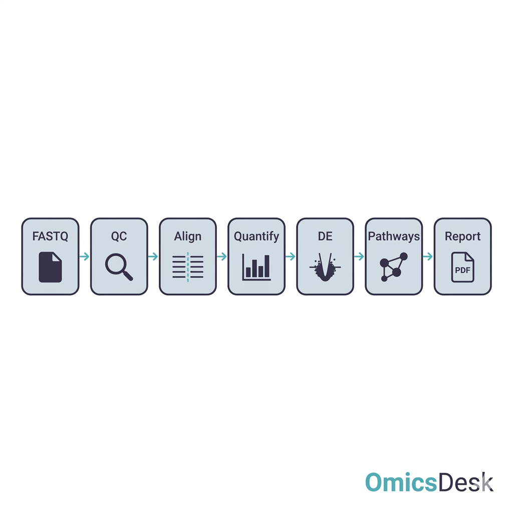
End-to-end RNA-seq workflow: QC, alignment, quantification, DESeq2, pathway analysis, reporting. The five stages, the real tool choices, and what production looks like in Snakemake.
You have a folder of FASTQ files. The sequencing facility delivered last week, the wet-lab side is celebrating, and someone — probably you — is now expected to produce a differential expression table, a list of pathways, and a figure your PI can put in a grant.
If you’ve never built an RNA-seq pipeline before, the next question is some version of “where do I start?”. If you’ve built one before, the question is closer to “do I really want to do this again?”
This is a tour of what an RNA-seq pipeline actually looks like when it’s run properly in 2026 — five stages, roughly ten real tool decisions, and a few traps that show up only in week three. The aim is not to teach you any single tool; the docs for each are excellent. The aim is to make the scope honest, so you can decide whether to invest two weeks in doing it carefully, or hand it to someone whose job this is.
You have FASTQ files. What now?
Bulk RNA-seq from raw reads to a DE table is five stages, in this order:
- QC and trimming — is the library good enough to bother analysing?
- Alignment or pseudoalignment — assign reads to a reference.
- Quantification — turn alignments into gene-level counts.
- Differential expression — model the counts and test contrasts.
- Functional analysis and reporting — turn a gene list into something interpretable, and package the whole thing.
None of these stages can be skipped. The temptation is always to skip QC (“the facility said the data is fine”) or alignment QC (“my mapping rate is 90%, that’s good, right?”), and the cost of doing that shows up later when DE results look weird and you can’t tell whether the biology is real or a technical artefact.
The whole thing needs to be wrapped in something reproducible — typically Snakemake or Nextflow. We’ll come back to that.
Stage 1: QC and trimming (fastp)
The job at this stage is to find out whether the raw data is salvageable, and to clean off the technical artefacts that would mess up alignment if left in.
The dominant single-tool choice in 2026 is fastp. It does adapter trimming, quality trimming, polyG/polyX trimming (important for NovaSeq two-colour chemistry), duplication detection, and per-sample HTML reports in one pass. Fast, sensible defaults, and the HTML report is what you actually look at:
fastp \
  --in1 sample_R1.fastq.gz \
  --in2 sample_R2.fastq.gz \
  --out1 sample_R1.trim.fastq.gz \
  --out2 sample_R2.trim.fastq.gz \
  --json sample.fastp.json \
  --html sample.fastp.html \
  --detect_adapter_for_pe
What you’re looking for in the report:
- Q30 percentage — at least 85% of bases above Q30. Below that, alignment will struggle.
- Adapter content — fastp will tell you if adapters were detected and trimmed. If it didn’t detect them, you may have the wrong adapter sequences for your library kit.
- Duplication rate — high duplication (>40%) on stranded poly-A libraries usually means the library was over-amplified or under-input.
- Insert size distribution — should peak somewhere reasonable (150–400 bp for most kits). A long tail at zero is adapter dimers that survived trimming.
There’s a host-specific gotcha on macOS arm64: fastp --thread N with N > 1 occasionally hangs after a few sequential calls in the same Snakemake DAG. Pin --thread 1 on that host or use Linux for batch jobs.
Stage 2: Alignment (STAR or pseudoalignment with Salmon)
You’re choosing between two paradigms.
STAR does true splice-aware alignment and produces a BAM where every read has a coordinate. You want this whenever you might need the BAM for anything beyond gene-level counts — variant calling from the RNA, splice-junction analysis, IGV inspection of specific loci. The cost is RAM: a human-genome index needs ~30 GB resident, and you need disk for the BAMs.
STAR \
  --runMode alignReads \
  --runThreadN 8 \
  --genomeDir refs/star_index/ \
  --readFilesIn sample_R1.trim.fastq.gz sample_R2.trim.fastq.gz \
  --readFilesCommand zcat \
  --outSAMtype BAM SortedByCoordinate \
  --outFileNamePrefix aligned/sample. \
  --quantMode GeneCounts
Salmon (pseudoalignment) does transcript-level quantification directly from FASTQ, without a coordinate-resolved BAM. Much faster (10–15 min per sample vs. ~45 min for STAR), far less RAM, and for gene-level DE it gives results that are statistically equivalent. You lose the BAM, which means no variant calling and no per-locus visualisation downstream.
salmon quant \
  -i refs/salmon_index/ \
  -l A \
  -1 sample_R1.trim.fastq.gz \
  -2 sample_R2.trim.fastq.gz \
  -p 8 \
  --validateMappings \
  -o quants/sample/
The default rule of thumb: STAR when the project might need variant calling or splice analysis later, Salmon when it’s purely “give me a DE table.” Make this choice once per project, write it down.
A trap to know: if you’re running STAR, check Log.final.out for % Uniquely mapped reads. Below ~70% on a vertebrate sample usually means rRNA contamination, severe degradation, or — most often — the wrong reference. Mismatched assembly versions (GRCh38 vs. GRCh37) and missing decoys are the silent killers.
Stage 3: Quantification (featureCounts / tximport)
If you went the STAR route, featureCounts (from the Subread package) turns a sorted BAM into per-gene counts using a GTF:
featureCounts \
  -a refs/Homo_sapiens.GRCh38.110.gtf \
  -o counts.tsv \
  -p --countReadPairs \
  -s 2 \
  -T 8 \
  aligned/*.sorted.bam
The flag -s 2 says “reverse-stranded library.” This is correct for most modern kits (Illumina TruSeq Stranded, NEBNext Ultra II Directional). Get it wrong and you’ll lose roughly half your counts to “the other strand” — and you may not notice if you don’t plot the count distribution.
If you went the Salmon route, you import the transcript-level quants into R with tximport and roll them up to gene level:
library(tximport)
tx2gene <- read_tsv("refs/tx2gene.tsv")
txi <- tximport(salmon_files, type = "salmon", tx2gene = tx2gene)
Either way, you end up with a counts matrix (genes × samples). That matrix is the input to DE.
Stage 4: Differential expression (DESeq2 — design formula matters more than tool choice)
DESeq2, edgeR, and limma-voom are all production-grade. For most projects, DESeq2 is the default — well-supported, conservative, and the visualisation ecosystem around it is the strongest.
The single most important decision at this stage is not the package. It’s the design formula:
library(DESeq2)
dds <- DESeqDataSetFromMatrix(
  countData = counts,
  colData   = metadata,
  design    = ~ batch + condition
)
dds <- DESeq(dds)
res <- results(dds, contrast = c("condition", "treated", "control"))
Three things go wrong here, in increasing order of how painful they are:
- You forgot a covariate. Sex, batch, library prep date. DESeq2 doesn’t read minds — if it’s not in
design, the variance ends up in the residual and your power drops. - You included a covariate that’s confounded with condition. If all your “treated” samples were prepped on Day 1 and all your “control” on Day 2, you cannot separate condition from batch and the model will silently struggle.
- You skipped the PCA. PCA before
DESeq()takes 30 seconds and catches mislabels, technical outliers, and conditions that aren’t the dominant variance source. We wrote a whole post on why PCA before DE is non-negotiable.
After fitting, shrink the log-fold-changes — raw LFCs from DESeq2 are noisy for low-count genes:
res_shrunk <- lfcShrink(dds, coef = "condition_treated_vs_control", type = "apeglm")This is what should go on volcano plots and ranked gene lists, not the raw res$log2FoldChange.
Stage 5: Functional analysis and reporting
A list of 3,000 significant genes is not a deliverable. The two things you do next:
- Pathway / enrichment analysis. GO, KEGG, Reactome enrichment via clusterProfiler. The mode matters: over-representation analysis (ORA) if you have a discrete significant-gene list, GSEA if you have a ranked list. They are not interchangeable.
- TF activity inference. Tools like DoRothEA + decoupleR project the DE signature onto regulatory networks and tell you which transcription factors are likely driving the observed changes. This is often the most interpretable layer for a biologist who doesn’t want to scan gene lists.
Then it has to be packaged. At minimum:
- A branded PDF report with executive summary, QC overview, PCA, volcano, top-hits table, pathway plots, TF activity, conclusions.
- An Excel workbook with one sheet per result class — full DE table, significant genes, pathway hits, TF activities — so the biologist can filter and sort without learning R.
- All figures as separate high-resolution PNG/SVG, ready for posters and slides.
This stage is where most DIY pipelines stop being reproducible. People generate figures in interactive R sessions, save them, and a month later can’t regenerate them when the metadata changes. The fix is to render the whole report from the analysis output — at OmicsDesk we use Quarto with a parameterised template, so the same Snakefile produces the same PDF every time.
Why Snakemake (the dry-run is the killer feature)
Once you have five stages, three tools per stage, twenty samples, and a couple of references, running it manually is a recipe for one of those Monday-morning “wait, which version of this did I send the PI?” moments. You need workflow management.
Snakemake and Nextflow are both fine. We use Snakemake at OmicsDesk because:
- It’s Python, so the engineers who write the analysis can extend the pipeline.
snakemake --dry-runprints exactly which rules will execute and which inputs they depend on, before anything runs. This is the killer feature: change a config value, dry-run, and see precisely which jobs need to re-run.- Conda integration is first-class — every rule can pin its own environment, so the QC step doesn’t fight the DE step over package versions.
- Reports are first-class too —
snakemake --reportproduces a self-contained HTML with the DAG, runtimes, and provenance for every output.
The one command to run the whole thing:
snakemake --use-conda --cores 8 --conda-prefix ~/snakemake_envs(On macOS, build the conda envs on an APFS volume — not on an exFAT external drive. AppleDouble metadata files corrupt heavy conda envs and the failure mode is silent.)
The honest tradeoff: DIY vs. hand off
If you got this far and thought “OK, I can do this,” you probably can. Two weeks of careful work, plus another week of fixing things you find when the biologist looks at the report and asks the first sharp question.
If you got this far and thought “I have eleven other things to do this month,” that’s also valid. The economics of doing this once or twice a year in-house are bad — you build expertise, lose it between projects, rebuild it next time, and never quite get to the production-grade version because every project is also fighting fires elsewhere.
What we run at OmicsDesk is exactly the pipeline described above — fastp → STAR/Salmon → featureCounts/tximport → DESeq2 → clusterProfiler + decoupleR → Quarto. Snakemake-wrapped, conda-pinned. Two hours of human review on top of every automated run, so the PCA gets real eyes before DE fires and the report tells a coherent story.
If you have FASTQ files sitting on a server and you want this run for you, upload them at submit.omicsdesk.com. The intake agent confirms the analysis plan with you — design formula, contrasts, what gets reported — before any compute starts. You get back a branded PDF plus an Excel workbook in 7–10 business days. Fixed price per omics type, no retainer, no new hire.
If you’re building this in-house and you have a specific question on any of the five stages, the comments are open.