PCA for Batch Diagnosis: What the Plot Is Telling You and What to Do Next

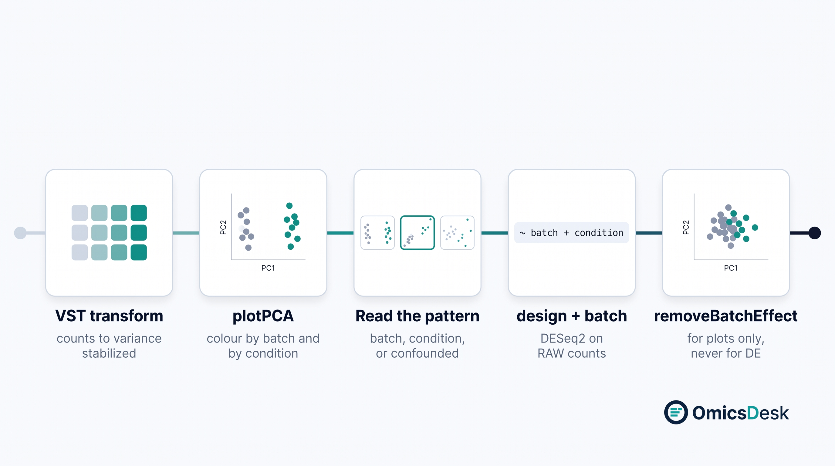
You ran PCA on your bulk RNA sequencing data. Something looks off: the samples are not grouping the way you expected. Before you start troubleshooting the biology, check whether the grouping is a technical artifact. PCA is the fastest, most reliable way to find out. If you have not run it yet, start with why PCA belongs before differential expression; this post is what to do once the plot already looks wrong.

Why PCA is the right first diagnostic

PCA reorders the variance in your data. The first principal component (PC1) captures whatever is responsible for the largest spread across samples. If your experiment is clean, PC1 should reflect the biological condition you care about. If it reflects something else, you have found a source of unwanted variation.

The standard approach: normalize your counts (VST or rlog in DESeq2), run plotPCA, then color the same plot two ways: once by biological condition, once by any known technical variable (batch, sequencing date, RNA extraction plate, lane).

If your samples cluster differently depending on which color you use, that technical variable is explaining a large chunk of the variance. That is not automatically a disaster. It is a diagnosis.

Three patterns and what they mean

Pattern 1: Condition drives PC1, batch is scattered. Your biological signal is the dominant source of variance. Batch effects exist (they always do) but they are small enough that the experiment can proceed. Still add batch to your DESeq2 model if you know the batch labels.

Pattern 2: Batch drives PC1, condition drives PC2, and the batches are balanced. “Balanced” means each batch contains samples from both conditions. This is the fixable case. The batch effect is real and large, but because it is not entangled with your biology, you can model it out.

Pattern 3: Batch drives PC1, and every sample in batch A is condition A. This is the confounded case. You cannot tell whether a gene is differentially expressed because of the biology or because of the technical difference between the batches. No statistical correction can fix this. This is a design problem.

What to do: the balanced batch

Add batch as a covariate in your DESeq2 design formula:

dds <- DESeqDataSetFromMatrix(
  countData = counts,
  colData   = metadata,
  design    = ~ batch + condition
)

That is almost always the right first move. DESeq2 will partition out the batch variance before estimating the condition effect. The result is the same number of samples, the same counts, but a model that accounts for the known technical structure.

If you want to visualize your data without the batch effect (for PCA or heatmaps), use limma::removeBatchEffect on VST values. That gives you a clean plot. The key rule: use the corrected values for visualization only. Do not run DE on them.

What NOT to do: running DE on batch corrected counts

This comes up often. Someone runs ComBat seq to remove the batch, takes the corrected count matrix, feeds it back into DESeq2, and reports the results.

The problem: ComBat seq assumes a negative binomial model and adjusts the counts. When you then feed those adjusted counts into DESeq2, DESeq2 tries to estimate dispersion on data that has already been transformed. The statistical assumptions no longer hold. You will get inflated significance and false positives.

The correct split: correction in the model (DESeq2 design), visualization on corrected values only (limma removeBatchEffect or ComBat on VST), DE always on raw counts with the full model.

When you are stuck: the confounded batch

If your PCA shows confounded batch, the honest answer is that the data has a structural limitation. A few options depending on your situation:

• If you have additional samples from the underrepresented conditions in each batch, add them.
• If resequencing is possible, do it with the batches crossed.
• If neither is possible, document the confound explicitly in the methods and interpret the DE results with appropriate caution.

There is no statistical method that reliably separates a batch effect that is perfectly correlated with the condition you are studying. Acknowledge it rather than papering over it.

A quick recipe

1. VST-transform your counts.
2. Run plotPCA(vsd, intgroup = "condition") and plotPCA(vsd, intgroup = "batch").
3. Decide which pattern you are in (1, 2, or 3 above).
4. If balanced: add + batch to your design, run DESeq2 on raw counts.
5. For visualization: use limma::removeBatchEffect(assay(vsd), batch = metadata$batch).
6. Never feed ComBat output back into DESeq2 for DE.

PCA is the first five minutes of every RNA seq QC. Knowing how to read it means you spend the next five minutes on the right fix, not the wrong one.

If you are not sure which pattern your data falls into, or whether your design can support a reliable correction, DM me. Happy to take a look.