Class I phosphosites: the filter that changes everything in phosphoproteomics

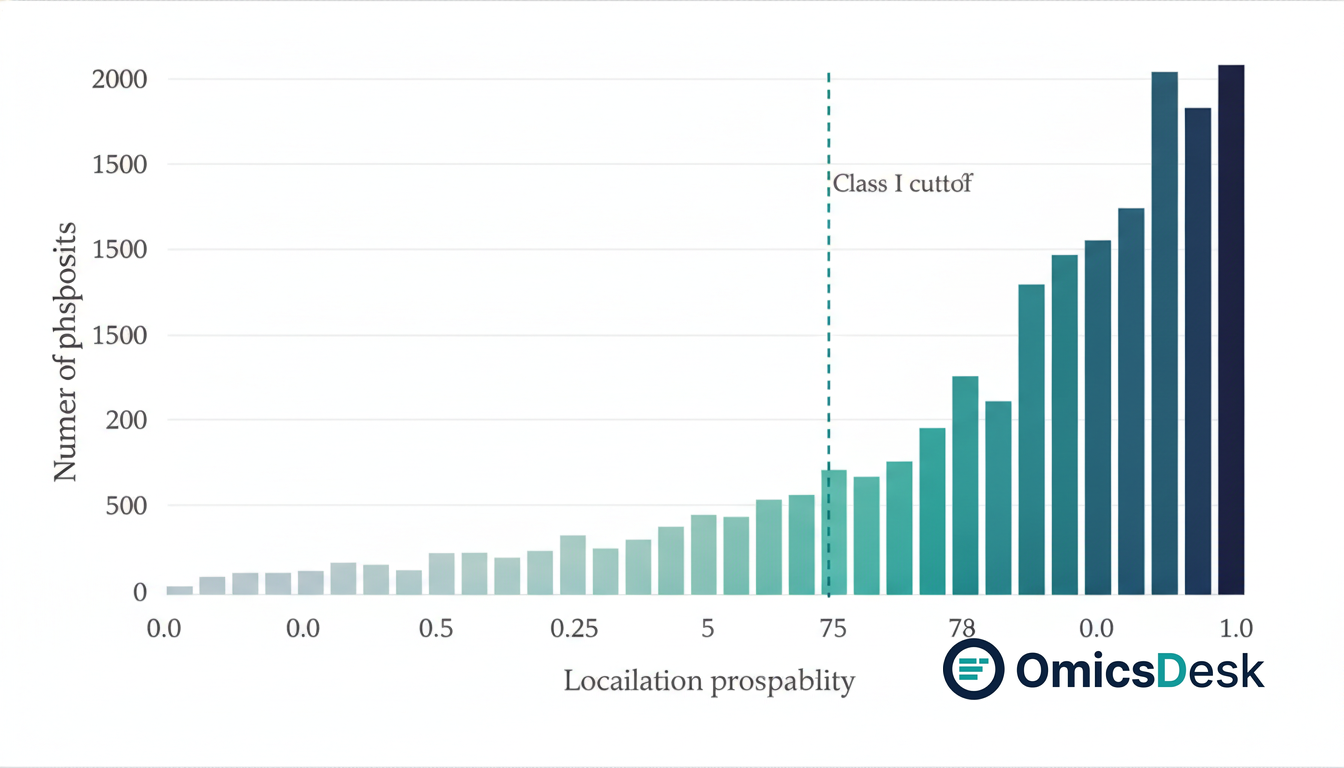
You get your MaxQuant output and see 12,000 phosphosites. You run differential abundance and get 800 hits. Then your reviewer asks: “How many of those sites are confidently localized?”

You check. About 3,500 of the 12,000 sites have a localization probability below 0.75. You never filtered them.

This is the most common silent quality failure in phosphoproteomics. Here is what localization probability means, what Class I, II, and III are, and how to fix it in one line of code.

What localization probability actually measures

Tryptic peptides from a phosphoproteomics experiment often contain more than one serine, threonine, or tyrosine residue. The mass spectrometer can detect that one of them is phosphorylated, but the fragment ions sometimes do not give enough information to say which one.

Localization probability (LP) is the probability that the phospho group sits on the reported residue and not on a nearby candidate within the same peptide window. A score of 100 means the assignment is unambiguous from the fragment spectrum. A score of 5 means the site could be on any of several residues and the algorithm essentially guessed.

The scoring comes from PhosphoRS (MaxQuant), PTMProphet (FragPipe), or the equivalent in Spectronaut. The math is a Bayesian model over all possible phospho configurations and their match to the observed MS2 spectrum.

A key property: LP is calibrated per-spectrum, not per-experiment. Two peptides with LP = 80 have roughly the same probability of correct assignment regardless of which run they came from.

Class I, II, III: what the thresholds mean

The three-class system follows the Olsen lab convention (Olsen 2006, Nat Methods) and is the standard in the field:

Class	Localization probability	Interpretation
Class I	> 0.75	High confidence: the site is correctly assigned with >75% probability
Class II	0.50 to 0.75	Moderate: the assignment is plausible but not definitive
Class III	< 0.50	Low: the site is ambiguously assigned; the true residue is unknown

In a typical label-free DDA phosphoproteomics dataset, roughly 60 to 75% of identified sites are Class I. Another 15 to 20% are Class II, and 10 to 15% are Class III. The exact proportions depend on the instrument, the fragmentation method (HCD vs ETD), and peptide length.

The threshold at 0.75 is a community convention, not a hard biological cutoff. Some groups use 0.90 for high-confidence datasets or for specific residue types (e.g. tyrosine phosphorylation, which is rare and deserves stricter criteria). The 0.75 cutoff is a reasonable starting point and the one your reviewers will expect to see.

Why Class II/III inflate false positives in differential analysis

If you run site-level differential abundance on unfiltered phosphoproteomics data, roughly 25 to 40% of your input “sites” are ambiguously assigned. What that means in practice:

A Class III site does not represent one biological phosphorylation event. It represents a peptide with a detected phospho modification that could be at residue S234, T237, or S241: the experiment cannot tell you which one. When you compare treated vs control, you are computing the log2FC of a mixture of three possible modifications. The result is a number that has no interpretable biological meaning.

Olsen and colleagues showed in 2010 that the differential abundance of many Class II/III sites reflects the parent peptide being differentially abundant, not site-specific regulation. The signal is real; the site annotation is wrong. The consequence is an inflated hit list where a portion of your “phospho-regulated” sites are false positives in the site-assignment sense, not the statistical sense.

This is separate from the FDR you control with the decoy database. You can have LP = 0.20 and a PSM q-value of 0.001. The identification is confident; the site assignment is not.

How to filter in practice

The filter is one line in R or Python. The column name differs by software:

MaxQuant (Phospho(STY)Sites.txt):

sites <- sites[sites$Localization.prob >= 0.75, ]

FragPipe (psm.tsv, MaxProbability column):

sites <- sites[sites$MaxProbability >= 0.75, ]

Spectronaut (EG.PTMLocalizationProbabilities):

sites = sites[sites["EG.PTMLocalizationProbabilities"] >= 0.75]

Apply this filter before any normalization, imputation, or differential analysis step. The resulting matrix is your working dataset. Every downstream analysis operates on this filtered set only.

If you are using the OmicsDesk phosphoproteomics pipeline, the filter is controlled by localization_prob_threshold: 0.75 in config.yaml. The pipeline applies it at the earliest possible step and logs how many sites were removed at each class level.

What to do with the discarded sites

Do not silently discard Class II and III sites. A fraction of them are biologically real phosphorylation events that happen to occur on peptides where the MS2 evidence is weak, either because of poor fragmentation coverage or because two candidate residues are very close together.

The right approach:

1. Keep a separate “discarded sites” table in the results workbook with columns for peptide, candidate residues, LP score, and parent protein.
2. Before reporting a hit from the Class I analysis, check whether the same peptide also has a Class II/III entry. If yes, note it as an ambiguous locus in the report.
3. If a Class II/III site hits a known regulatory residue in PhosphoSitePlus or is biologically motivated by prior literature, flag it for orthogonal validation (mutagenesis, phospho-specific antibody). Do not include it in the primary statistics, but do not pretend it does not exist.

This approach keeps the primary analysis clean while not throwing away potentially interesting biology.

The bottom line

Every phosphoproteomics analysis should start with the Class I filter. It takes one line. It removes a meaningful fraction of noise from the differential analysis and makes your hit list interpretable. If you inherited a dataset that was analyzed without this filter, the first step is to re-run the differential analysis on the filtered matrix and see how many hits survive.

A shorter hit list with confident site assignments is more useful than a longer list where a third of the entries may be on the wrong residue.

If you need a phosphoproteomics analysis run correctly from raw files to a filtered site-level DE table, DM me. That is exactly what OmicsDesk delivers.