GSEA vs over-representation analysis in RNA-seq: why your DEG list misses pathways GSEA still finds

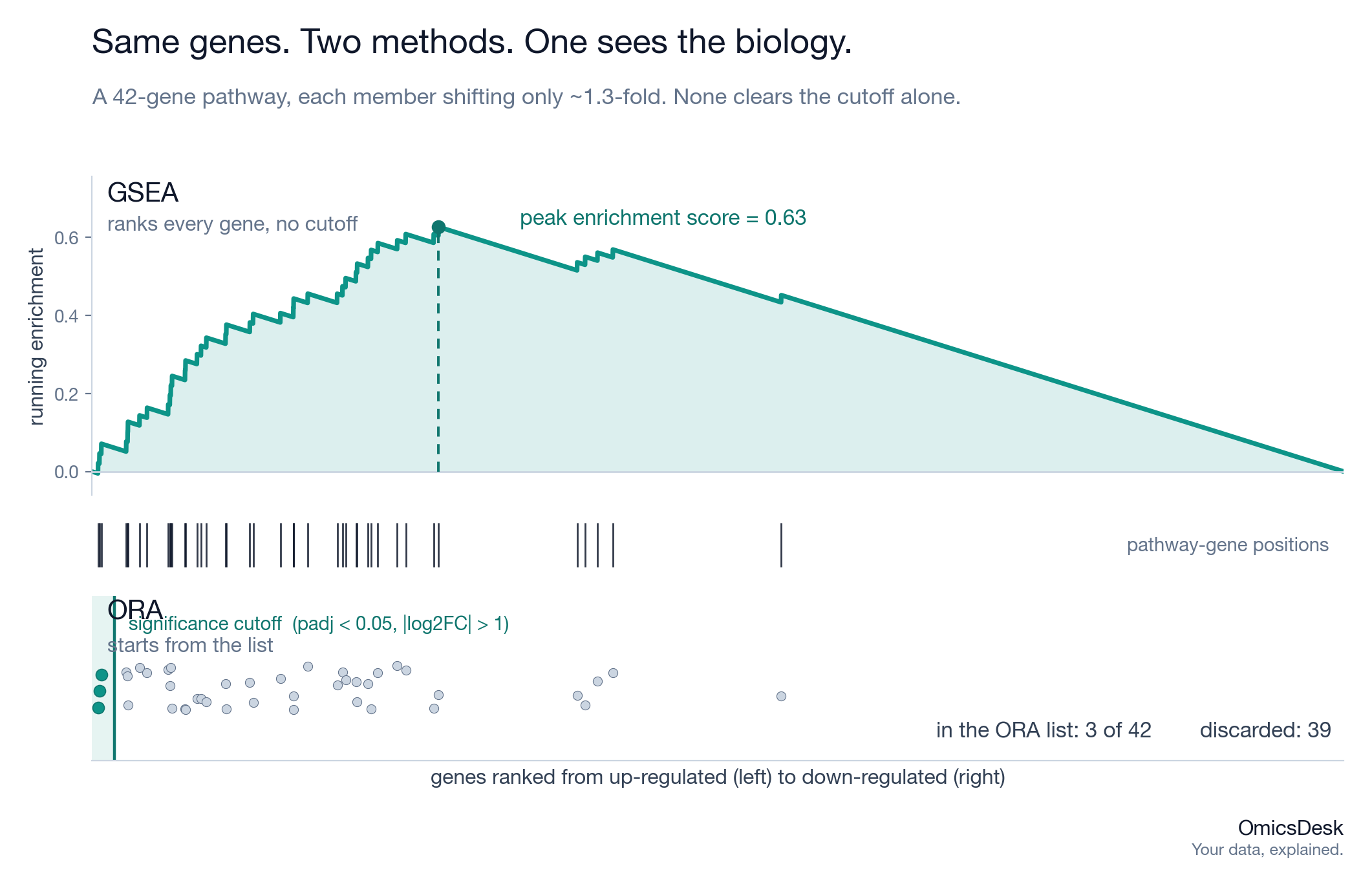
Your top 30 genes all missed the significance cutoff. The pathway analysis came back empty. The wet-lab side concludes the experiment found nothing. Then you run the same contrast through GSEA and a coherent pathway lights up at an FDR you can defend. Nothing changed about the data. What changed was whether the method was allowed to look at the genes you had thrown away.

This post is about the choice between two enrichment methods that get used interchangeably and should not be: over-representation analysis (ORA, the enrichGO / DAVID / clusterProfiler style that takes a gene list) and gene set enrichment analysis (GSEA, the ranked-list style). They answer different questions, they fail in different ways, and on heterogeneous data they routinely disagree. If you analyse RNA-seq where effect sizes are modest, picking the wrong one is the difference between a result and a dead end.

What over-representation analysis actually does

ORA starts from a list. You run differential expression, apply a cutoff (say padj < 0.05 and |log2FC| > 1), and you are left with, say, 80 genes. ORA asks one question of that list: are any pathways represented more often than you would expect by chance? It builds a 2x2 contingency table per gene set (in your list or not, in the pathway or not) and runs a hypergeometric or Fisher test.

The mechanic that matters is in the first sentence: it starts from a list. Every gene that did not clear the cutoff is invisible to ORA. A gene at padj of 0.06 contributes exactly as much as a gene that was never sequenced, which is nothing. You have compressed a ranked, quantitative result down to a binary membership flag, and then asked a question about the flags.

That compression is fine when the list is the point. If you have 200 ChIP-seq peaks, or a curated panel of validated hits, the genes really are a discrete set and ORA is the honest tool. The trouble is using it on RNA-seq, where the “list” is an artifact of a threshold you chose, not a property of the biology.

What GSEA does differently

GSEA never makes a list. It takes every gene in the experiment, ranks them from most up-regulated to most down-regulated by a single metric, and then asks, for each gene set, whether its members are clustered toward the top or bottom of that ranking rather than scattered randomly through the middle. It walks down the ranked list keeping a running enrichment score that climbs when it hits a pathway member and decays otherwise; the peak of that walk is the enrichment score, and a permutation test gives it a p-value.

No cutoff is applied. No gene is discarded. A gene at padj of 0.06 sits exactly where its statistic puts it in the ranking and contributes its full weight. That single design difference is the whole reason the two methods diverge.

Why GSEA finds biology ORA misses

Consider a pathway of 40 genes where every member shifts by about 1.3-fold in the same direction, and none of them individually clears a 2-fold cutoff or a padj of 0.05. To ORA this pathway is invisible: zero of its genes are in the list, so the contingency table shows no enrichment. To GSEA the same pathway is obvious, because 40 genes all sitting in the top third of the ranking is wildly unlikely by chance, even though no single one of them would survive on its own.

This is the common case in patient tissue, not the exception. Human samples are heterogeneous, the contrasts are rarely clean on/off switches, and coordinated programs often move as a crowd of small, consistent shifts rather than a handful of large ones. ORA is built to reward the handful of large shifts. GSEA is built to detect the crowd. When your DEG list is short and your biology is real but diffuse, that is exactly when the two methods disagree, and GSEA is usually the one telling the truth.

The two choices that decide whether it works

GSEA is not automatic. Two decisions determine whether the result is signal or garbage.

The ranking metric. GSEA is only as good as the ordering you hand it. The robust default is the sign of the fold change multiplied by a significance term, for example sign(log2FC) * -log10(pvalue), or the stat column straight out of DESeq2, which already encodes both. Ranking by raw fold change alone is the classic mistake: a gene at 8-fold with two noisy replicates and a padj of 0.4 should not outrank a gene at 1.5-fold that is rock solid, but on a fold-change ranking it does, and it drags noise to the top of your list where GSEA weights it most.

library(fgsea)

# DESeq2 already gives you a signed, significance-aware statistic.
res <- results(dds)
ranks <- res$stat
names(ranks) <- rownames(res)
ranks <- sort(ranks[!is.na(ranks)], decreasing = TRUE)

fgseaRes <- fgsea(pathways = hallmark, stats = ranks,
                  minSize = 15, maxSize = 500)

Clean gene sets. Run one collection at a time. Throwing Hallmark, GO biological process, and KEGG into a single call inflates the multiple-testing burden and, worse, gives you overlapping, redundant hits that look like ten findings but are one program described in three vocabularies. Pick the collection that matches your question, set minSize to drop tiny sets that pass on three genes of noise, and cap maxSize so a 2000-gene “metabolism” bucket does not pass on sheer breadth.

When ORA is still the right tool

This is not an argument that GSEA wins every time. ORA is the correct choice whenever your input genuinely is a discrete set with no meaningful internal ranking: peaks from a ChIP-seq or ATAC-seq experiment, a hand-curated panel, the members of a co-expression module, the genes inside a copy-number segment. In those cases there is no whole-transcriptome ranking to feed GSEA, and forcing one would be inventing structure that is not there. The rule of thumb is simple. If you have a ranked statistic for every gene, use GSEA. If you have a list and nothing behind it, use ORA, and do not pretend the list was not a choice.

How to read the output

A GSEA result table has a handful of columns that carry the decision. Read them in this order.

The normalised enrichment score (NES) is the headline. Its sign tells you direction (positive means the set is enriched among up-regulated genes, negative among down-regulated), and its magnitude is comparable across gene sets of different sizes, which the raw enrichment score is not. The padj (or FDR q-value) is your significance gate; with a permutation null and many sets tested, treat anything above 0.25 with suspicion and prefer sets under 0.05 when you can get them. The size column is a sanity check: a set that passed on 8 genes out of a nominal 300 is fragile, and minSize/maxSize should have caught it.

The column people skip and shouldn’t is the leading edge, the subset of genes that occur before the running score hits its peak. Those are the genes actually driving the call. If a pathway is significant but its leading edge is three housekeeping genes you recognise, the result is real arithmetic and useless biology. Always read the leading edge before you write the sentence that goes in the report.

The misuses that quietly ruin the result

Three mistakes show up again and again.

First, filtering by p-value and then running GSEA on the survivors. This is the worst of both worlds: you have thrown away the lower half of the ranking that GSEA needs, then asked a ranked method to work on a truncated list. GSEA takes the whole transcriptome on purpose. Give it the whole transcriptome.

Second, mixing gene-set collections in one run, covered above. It feels thorough and reads as inflated.

Third, ranking on the wrong metric, also above, usually raw fold change. If your top GSEA hits look biologically random, check the ranking before you check the biology.

Get those three right and GSEA does something ORA structurally cannot: it tells you about the coordinated, modest shifts that are most of what real tissue actually does.