MOFA2 Explained: Integrating RNA-seq, Proteomics, and ATAC-seq in One Model

You ran RNA-seq and proteomics on the same 40 patient samples. RNA-seq gives you 800 differentially expressed genes. Proteomics gives you 200 differentially abundant proteins. The overlap between the two lists is about 60 features.

What about the other 940 features? Are they noise, or signal you missed by analyzing each layer in isolation?

This is the core problem of multi-omics integration. Each assay has its own noise structure, its own depth bias, and its own feature space. Intersecting hit lists at the end throws away signal from features that move together coherently but narrowly miss the per-assay threshold in any single modality. You need a method that looks across all layers simultaneously, from the start.

MOFA2 is one of the best tools for that.

The problem with analyzing each omics layer in isolation

When you run DESeq2 on your RNA-seq and limma on your proteomics separately, you are fitting two independent models. Each makes its own call about which features are significant. They only agree when the same biology is strong enough to clear both thresholds independently.

In practice, RNA-seq and proteomics hit lists from the same experiment typically overlap 20 to 30%, even in well-powered studies. The other 70 to 80% is not noise: some of it is genuinely discordant biology (post-transcriptional regulation, protein stability, translation efficiency), but a lot of it is signal that was just beneath the per-assay threshold in one layer.

Intersecting lists is also agnostic to correlation structure. Two features that move together coherently across both assays but never rank highly in either are invisible to list-based integration. A joint model sees them.

What MOFA2 actually does

MOFA2 (Multi-Omics Factor Analysis v2, Argelaguet et al. 2020) is a Bayesian group factor analysis model. The input is a named list of matrices, one per omics modality, with features in rows and samples in columns. The model learns a set of latent factors, where each factor is a weighted linear combination of features spanning all modalities simultaneously.

Think of a factor as a principal component that lives across all your omics at once, not inside any single one.

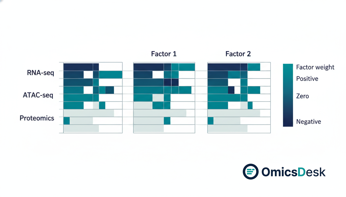
Each feature in each modality receives a weight on each factor. A large positive weight on Factor 1 means the feature tracks with whatever biological axis Factor 1 represents. A weight near zero means the feature is uninformative for that axis.

MOFA2 is fitted by variational Bayesian inference, not simple matrix decomposition. That matters for three reasons: it handles missing samples per modality (not every sample needs to be profiled in every assay), it handles different scales and distributions across modalities naturally, and it places sparsity priors on the weights so the solution stays interpretable rather than spreading signal across hundreds of features per factor.

Shared vs modality-specific factors

The most useful feature of MOFA2 is that not every factor loads on every omics layer.

The model uses automatic relevance determination (ARD) priors. If the features of a given modality do not explain a factor, the ARD prior shrinks all of that modality’s weights on that factor to zero. The modality drops out automatically.

In a joint RNA-seq and ATAC-seq and proteomics experiment, you might see something like:

Factor 1 loads strongly on both RNA-seq and ATAC-seq. This is a shared chromatin accessibility and transcription axis. It could be your treatment response, your differentiation gradient, or a technical batch effect that happened to affect both assays equally.

Factor 2 loads only on proteomics. This is a post-transcriptional regulation axis that RNA-seq cannot see. Protein turnover, protein complex assembly, and translational control are all invisible to transcript-level measurement. Without the proteomics layer, Factor 2 does not exist in your data.

Factor 3 loads only on ATAC-seq. An accessibility change that did not propagate to gene expression or the proteome. Primed chromatin for a later response, perhaps.

These distinctions are impossible to make from list intersections. They emerge naturally from the model.

MOFA2 vs DIABLO: when to use which

MOFA2 is unsupervised. It does not know about treatment groups, disease labels, or outcomes. It finds the axes of variance present in the data and tells you what biology each axis represents.

DIABLO (from the mixOmics R package) is supervised. You give it a class label (tumor vs normal, treated vs control) and it finds a multi-omics latent space that maximally discriminates those groups. It is a discriminant analysis, not a factor model.

Use MOFA2 when: you are exploring a cohort with no clean outcome label; some samples are missing from one or more modalities; you want to understand the full variance structure before fitting a supervised model; or you specifically want modality-specific factors alongside shared ones.

Use DIABLO when: you have a clear two-class or multi-class label and your primary goal is classification or supervised biomarker discovery; all samples are profiled in all modalities; and predictive performance is what you need to show.

Both are valid tools. They answer different questions. Many analyses benefit from running MOFA2 first (unsupervised exploration) and DIABLO second (supervised validation of the most informative factors).

What you get out

After training, MOFA2 outputs two key objects.

Factor scores (a samples x factors matrix): each sample gets a coordinate on each factor. Plot these like a PCA biplot, color points by your metadata (treatment, patient, time point, batch), and see immediately which factors separate your groups of interest. A factor that perfectly separates treated from control is biologically meaningful. A factor that separates by library preparation date is a technical artifact to regress out.

Factor weights (a features x factors matrix, one per modality): each feature has a weight on each factor. The top-weighted features are the ones driving that factor. Run gene set enrichment (GSEA, fgsea) on the top-weighted RNA-seq features of Factor 1 to get pathway interpretation. Do the same on the ATAC-seq peaks of Factor 1 (annotate peaks to genes, then run enrichment) and check whether the same pathways appear in both layers. When they do, that is one of the most confident findings you can report in a multi-omics study.

Factor scores also serve as covariates. If Factor 3 turns out to be a batch effect, include it in your downstream DESeq2 model to remove it more precisely than a categorical batch correction.

A minimal MOFA2 run in R

MOFA2 is on Bioconductor. Install with BiocManager::install("MOFA2"). For Python users, mofapy2 on PyPI and the muon ecosystem wrap it for scanpy workflows.

In R, the core workflow:

library(MOFA2)

# data_list: named list of matrices, features x samples, one per modality
# e.g. list(RNA = rna_vst_matrix, Proteomics = prot_log2_matrix, ATAC = atac_log_matrix)

mofa_obj <- create_mofa(data_list)

model_opts <- get_default_model_options(mofa_obj)
model_opts$num_factors <- 15   # 10 to 20 is a good starting range

train_opts <- get_default_training_options(mofa_obj)
train_opts$convergence_mode <- "medium"   # fast / medium / slow
train_opts$seed <- 42

mofa_obj <- prepare_mofa(mofa_obj,
  model_options   = model_opts,
  training_options = train_opts
)
mofa_obj <- run_mofa(mofa_obj, use_basilisk = TRUE)

Key inspection after training:

plot_variance_explained(mofa_obj)                       # % variance per factor per modality
plot_weights(mofa_obj, factor = 1, view = "RNA")        # top RNA features for Factor 1
plot_factor(mofa_obj, factors = c(1, 2), color_by = "condition")   # factor score biplot

For pathway enrichment, MOFA2 ships a fgsea wrapper:

enrichment <- run_enrichment(mofa_obj,
  feature.sets = hallmark_genesets,
  view = "RNA")
plot_enrichment(enrichment, factor = 1, max.pathways = 15)

One practical note on input preparation

MOFA2 expects pre-normalized data. For RNA-seq, use VST (variance-stabilizing transformation) from DESeq2 or log2-normalized CPM. For proteomics, log2-transformed LFQ intensities after missing-value filtering. For ATAC-seq, log-normalized peak counts. Raw counts will give poor results.

Feature selection also helps. Fitting MOFA2 on 25,000 expressed genes and 50,000 ATAC peaks is slow and the solution will be noisy. Select the top 5,000 to 10,000 most variable features per modality first. MOFA2 includes a select_features helper, or filter by per-feature standard deviation before passing the matrices in.

Training on a 40-sample three-modality dataset takes 5 to 15 minutes on a standard laptop with convergence_mode = "medium".

When multi-omics integration is worth it

Multi-omics integration adds the most value when no single assay can answer the biological question on its own. If you only need to know which genes change between conditions, RNA-seq is sufficient. If you want to know how chromatin accessibility drives those expression changes, you need ATAC-seq in the same samples. If you want to know whether the protein-level response matches the transcript-level response (it often does not, and the discordance is the interesting biology), you need proteomics.

The cost is sample complexity and computational overhead. MOFA2 benefits from at least 20 to 30 samples to estimate the covariance structure reliably. With n=3 per group, the factors will exist but the biological interpretation will be unstable across runs.

If you have a properly powered multi-omics cohort, MOFA2 is one of the most informative analyses you can run. The biology it surfaces is the kind that does not appear in any single-omics paper, because it requires looking across all the layers at once.

---

Running multi-omics integration on a real dataset? I run MOFA2 and DIABLO as part of the OmicsDesk multi-omics service, with a full report covering factor interpretation, pathway enrichment per modality, and publication-ready figures. Drop a brief at omicsdesk.com